Modeling Private Equity Market Beta

Over the past few decades, private equity and venture capital returns have been very robust, pushing many asset owners to increase their allocations. As their portfolios increasingly tilt towards private investments, getting the private portion right in terms of market exposure and risk becomes even more important.

A question we often get from clients is how best to model the stock market exposure of private equity. The process through which private equity returns are estimated makes modeling the asset class’ risk exposures challenging; namely, it dampens and smooths the volatility of private equity returns.

In this article, we will investigate how we can undo some of the risk dampening and smoothing inherent in private equity benchmark returns by accounting for the impact of lagged stock market returns on private equity.

The Impact of Smoothing on Returns

It’s hard to argue that private equity does not have at least some correlation to the public stock market. The standard indexes (such as those published by Cambridge Associates) used by asset owners to track private equity performance suffer from smoothing due to the subjectivity and lag inherent in the returns estimation process, which if unaccounted for, can cause private equity’s risk metrics (e.g. its stock market beta) to be understated. Thus, it is important to understand how smoothing impacts the statistical characteristics of private equity returns and to properly adjust for them.

This smoothing is the result of several factors.

First, many private equity funds update their valuations quarterly. It takes time for market declines to hit private equity portfolio company valuations. If the plunge and recovery happen quickly, like during last year’s COVID shock, the full impact of the decline may never ultimately flow through.

Second, private equity portfolio company valuations are often model or appraisal-based and therefore can be quite subjective due to inconsistent standards and methodologies. Third, investors tend to hold private equity investments to maturity given that private equities are less liquid and more costly to transact. Because estimated valuations aren’t used to transact, there is less incentive to get it right and significantly less signal to aid in doing so.

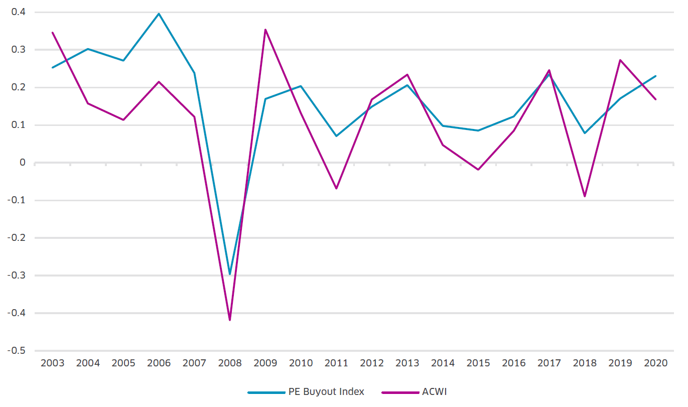
It is also worth noting that the performance fees charged by general partners (GPs) also serve to dampen observed volatility. During good times fees reduce gross returns, and during bad ones there are either no incentive fees or significantly reduced ones (bringing net returns closer to gross returns). You can see this dampened volatility (especially after 2008) in the plot below, which compares the annual returns of the Cambridge Private Equity Buyout Index (Buyout) to the All Country World Stock Market Index (ACWI).

We can use a simple linear regression (see equation below) to estimate private equity’s alpha and stock market beta. We will use the Cambridge Associates Private Equity Buyout Index as our estimate of asset class level private equity returns and the ACWI Index (All Country World Stock Market Index) as our proxy for the stock market. All the regressions in this article are run using quarterly returns from 1/1/2001 to the present.

PE Return = β0+β1 * M

PE Return = Quarterly returns of the Cambridge Associates PE Buyout Index
M = ACWI quarterly returns (unlagged)

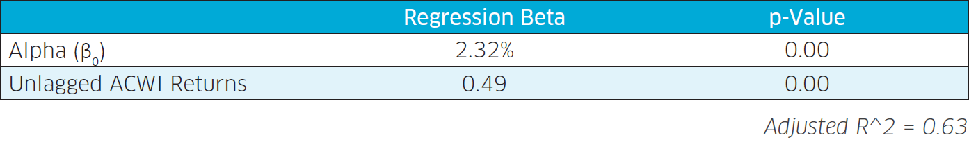
Examining the regression outputs, two things jump out.

First, private equity’s market beta is much lower than that of other risky assets such as small cap stocks or Emerging Market stocks (both of which have betas of more than 1.0). Second, since 2001, relative to its 0.49 stock market exposure, private equity has outperformed by on average 2.32% per quarter. While the full exploration of this is outside the scope of this article, it will be interesting to see how this alpha estimate changes after we account for private equity’s hidden market exposure.

In their 2001 paper “Do Hedge Funds Hedge?“, Clifford Asness, Robert Krail, and John Liew used a novel but intuitive approach to estimate stock market exposure in the presence of smoothing. In instances where lagged correlations to the market exist, they suggested summing the market betas (both lagged and unlagged) to get a more accurate estimate of stock market exposure. We will apply a similar approach to calculating private equity’s stock market beta

Calculating the “True” Stock Market Beta of Private Equity

We can augment our simple regression by including the ACWI’s quarterly lags using the following equation:

PE Return = β0+β1 * M+β2 * M(Lag,1)+β3 * M(Lag,2)+ … +βN * M(Lag,N-1)

PE Return = Quarterly returns of the Cambridge Associates PE Buyout Index
M = ACWI quarterly returns (unlagged)
M(Lag,t) = ACWI quarterly returns lagged by t quarters

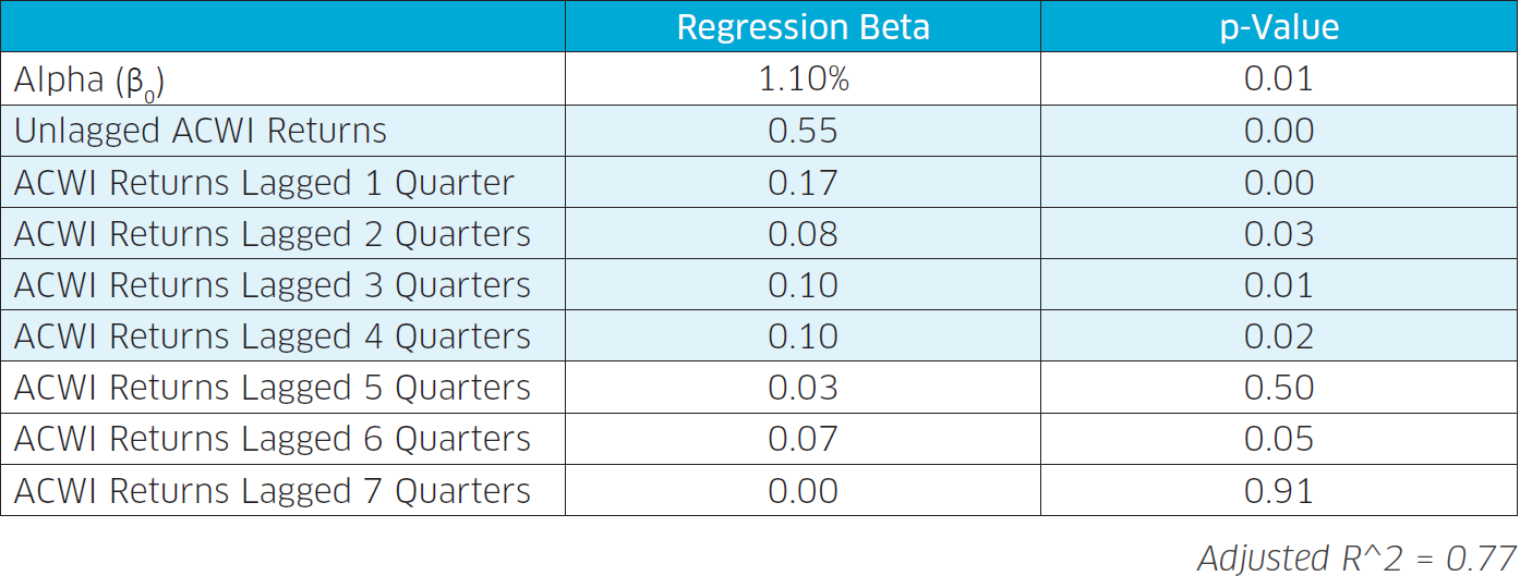
From the regression p-values (each of which measures the probability of seeing a beta of the observed magnitude purely due to random chance), we can see that several of the betas for the ACWI’s lagged quarterly returns are statistically significant at the 5% level. This result implies that the concurrent return of the stock market is not sufficient for estimating private equity’s market beta and that we must also consider the lagged returns as well. The shaded rows denote the betas that we ultimately decided to include in our model. The reason why we chose to include just four quarters of lag and not more is because the correlations observed at longer horizons are more likely to be spurious.

Because the ACWI and its lags are uncorrelated (see correlation matrix below), an investment with positive betas to both the concurrent return and several of its lags will see its volatility significantly dampened. This is no different than what happens when multiple uncorrelated return streams are combined in a portfolio; they will diversify and smoothen each other. Except in this case, the diversification is not real. We can’t actually invest in the lagged ACWI; it’s merely an accounting quirk.

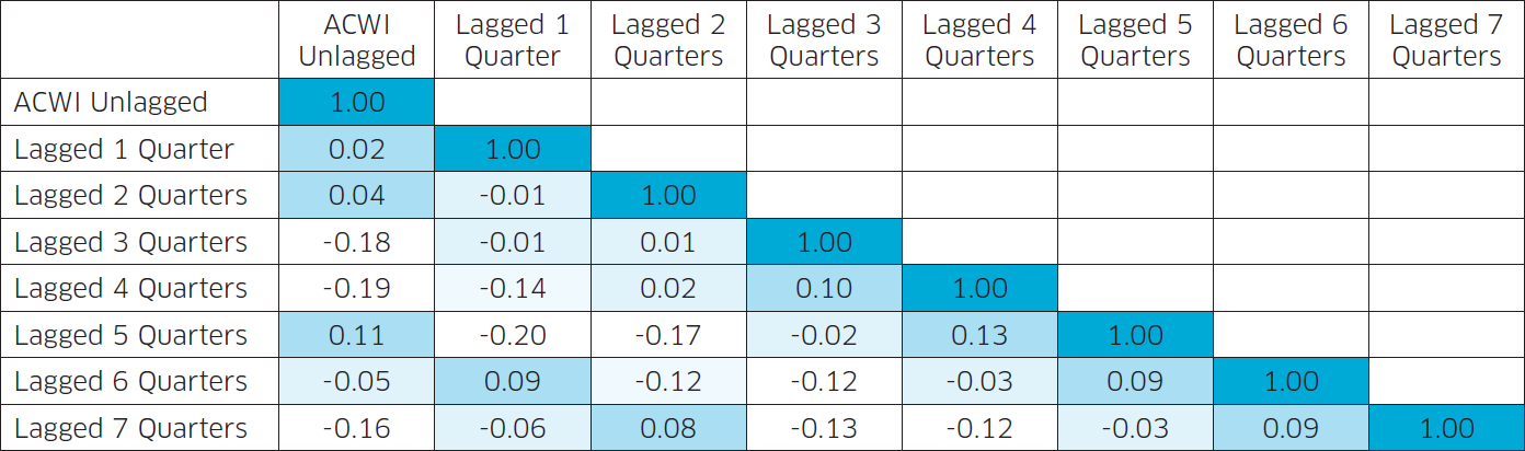
Because of these near zero correlations, we can simply sum the betas to the unlagged and lagged ACWI returns in order to obtain a truer market beta for private equity. As we are including only four lags, we need to rerun our regression with the following equation:

PE Return = β0 + β1 * M + β2 * M(Lag,1) + β3 * M(Lag,2) + β4 * M(Lag,3) + β5 * M(Lag,4)

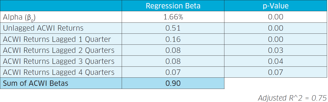
Summing the betas from zero to four lagged quarters produces a beta to the stock market of 0.90, significantly higher than the 0.48 beta estimated using just the concurrent return of the ACWI (a regression with no lags). This implies that there’s almost twice as much stock market risk embedded in private equity than initially meets the eye. Interestingly, even after accounting for the additional stock market exposure hidden in the lags, private equity returns still exhibit significant amounts of historical alpha over the period of analysis: down from 2.32% (calculated using just the concurrent ACWI return) to a still very attractive 1.66% alpha per quarter. No wonder that it’s become such a popular asset class among asset owners over the past few decades.

The Intuition Behind Summing the Betas

A key insight of this article is that summing the stock market betas, both concurrent and lagged, produces a truer estimate of private equity’s stock market exposure. It is worth examining a simplified (and hypothetical) case to firm up our intuition around why summing makes sense.

Imagine a case where a fund takes a quarter to complete its return calculations. On 12/31/2019, it starts gathering data on its underlying portfolio companies. It’s not until 3/31/2020 that it finishes and the fund can finally report the return of its portfolio that it realized over Q4 of 2019. The fund reports a return of 5% (because markets were doing fine at the end of 2019) despite public markets actually being in the midst of a significant decline due to the COVID pandemic. Without knowledge into the fund’s process, a benchmarking firm like Cambridge would have no way of knowing about the lag. Assuming our fund doesn’t volunteer the information, Cambridge would have no choice but to take that 5% at face value.

If we were to regress several years of returns for this fund (which we will call Fund A) against the concurrent returns of the S&P 500, we’d get a beta of around zero. Being thorough analysts, we try a second regression where we lag the S&P 500’s returns by a quarter. This second regression produces a beta of one, meaning that Fund A’s return is highly correlated to the S&P 500’s return from one quarter ago. In this case, the correct stock market beta for Fund A is not zero but one. The zero beta that we observed at first is an artifact of the fund’s process and not reflective of its actual economics.

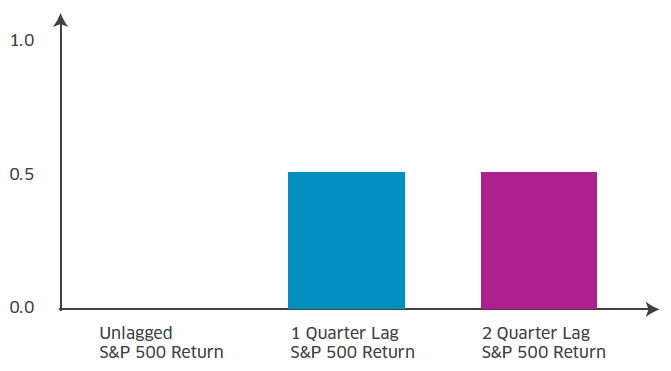
Now imagine there is a second fund, Fund B, with a more complicated portfolio and thus an even slower process that takes two quarters to produce results, giving it a beta of one to the S&P 500’s returns lagged by two quarters.

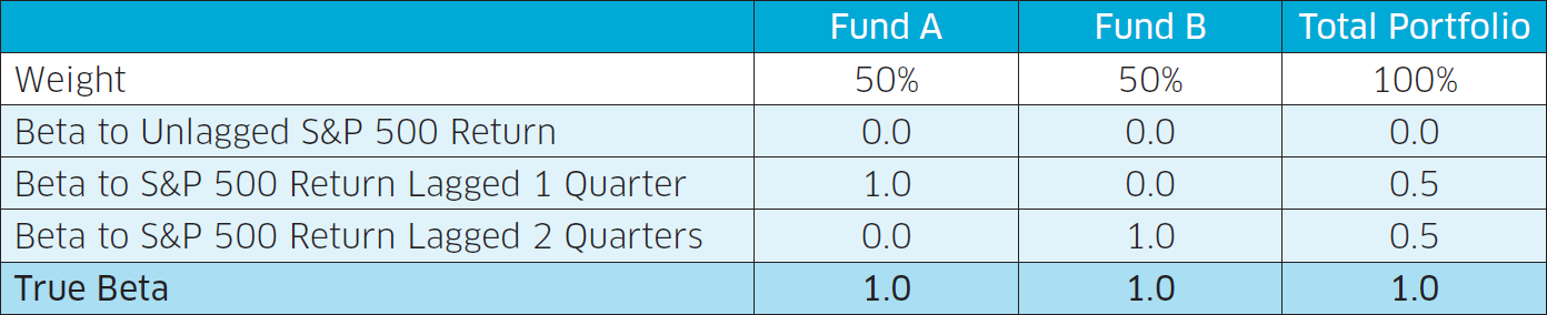
If we created a portfolio that allocated 50% to Fund A and 50% to Fund B, its stock market betas would look something like this (assuming little to no correlation between market lags).

In this case, the total stock market beta of our portfolio would be 0.5 + 0.5 = 1. Both Fund A and Fund B are actually highly correlated to the stock market. The market correlation and beta are masked by the varying degrees of lag in the two funds’ processes. Adjusting for these lags by taking a weighted sum of Fund A’s and Fund B’s betas to both unlagged and lagged S&P 500 returns produces the true portfolio beta:

Here’s how Asness, Krail, and Liew put it:

“In other words, we are trying to capture the fact that, assuming there is a real relation between the market and a hedge fund, when the market moves, the hedge fund should also move (e.g., if managers actually tried to sell their securities they would see this return immediately). Yet stale or managed pricing may prevent the move from fully showing up in the hedge fund’s reported returns in the same month. Instead, the move may show up slowly as securities are priced correctly in subsequent months. Thus, the hedge fund appears to move with the market at a lag.

The regression with lagged market returns measures the magnitude and statistical significance of this effect and provides a potentially more accurate beta estimate.”
– Asness, Krail, and Liew, 2001, pp 11

Conclusion

Regardless of whether it is private or public, an investment’s risk is driven by its underlying economic fundamentals. Getting these fundamentals right is critical to making good portfolio decisions. This approach underscores the importance of accounting for all risk factors, both apparent and hidden.

Nasdaq for Asset Owners

Nasdaq

Delivering insights and intelligence for institutional investors

Read Nasdaq for Asset Owners 's Bio